A knot is a circle inside \(3\)-dimensional space. A link is a collection of knots. Given a knot or link,
we can look at it from an angle and try to draw a line corresponding to what we see. However
whatever we see will not necessarily determine what our knot was, because the knot may cross
over itself when viewed from the angle we are looking at it from. To fix this, we also
need to put the crossing information in our drawing, namely whenever two strands pass
through each other, we need to say which strand goes above which other strand. Such a
drawing is called a projection of our knot or link. Examples of projections are shown
below:
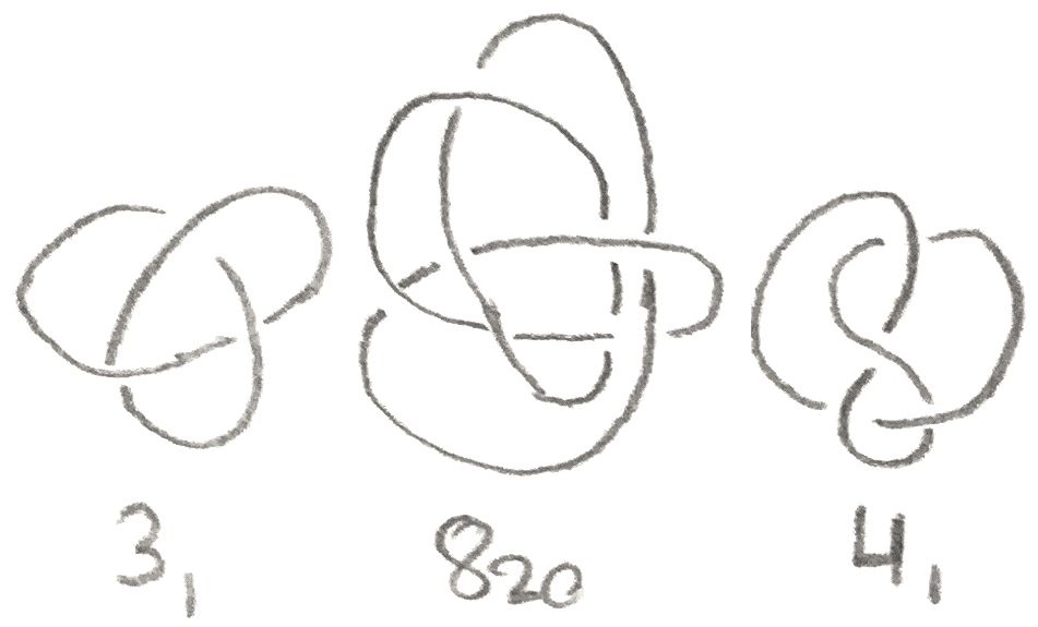
Figure 1:Some knots. \(3_1\) is also knot as the trefoil knot, and \(4_1\) is also known as the figure eight
knot
.
We say that two knots are equivalent if you can move around one knot without intersecting
itself to get the other. Knot theory is about studying knots up to equivalence. For example, the
knot below is not really knotted at all, indeed after moving it around, we can see that its
projection is a circle. This knot is called the unknot.
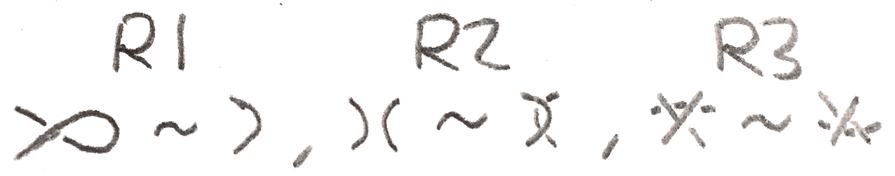
How can we go between projections of a knot? A theorem of Reidmeister says that apart from
moving around strands in ways that don’t affect the crossings, there are \(3\)-moves that get between
any two projections, shown in Figure 2.
Figure 2:
Thus if we want to study links, it suffices to study projections of links up to doing Reidmeister
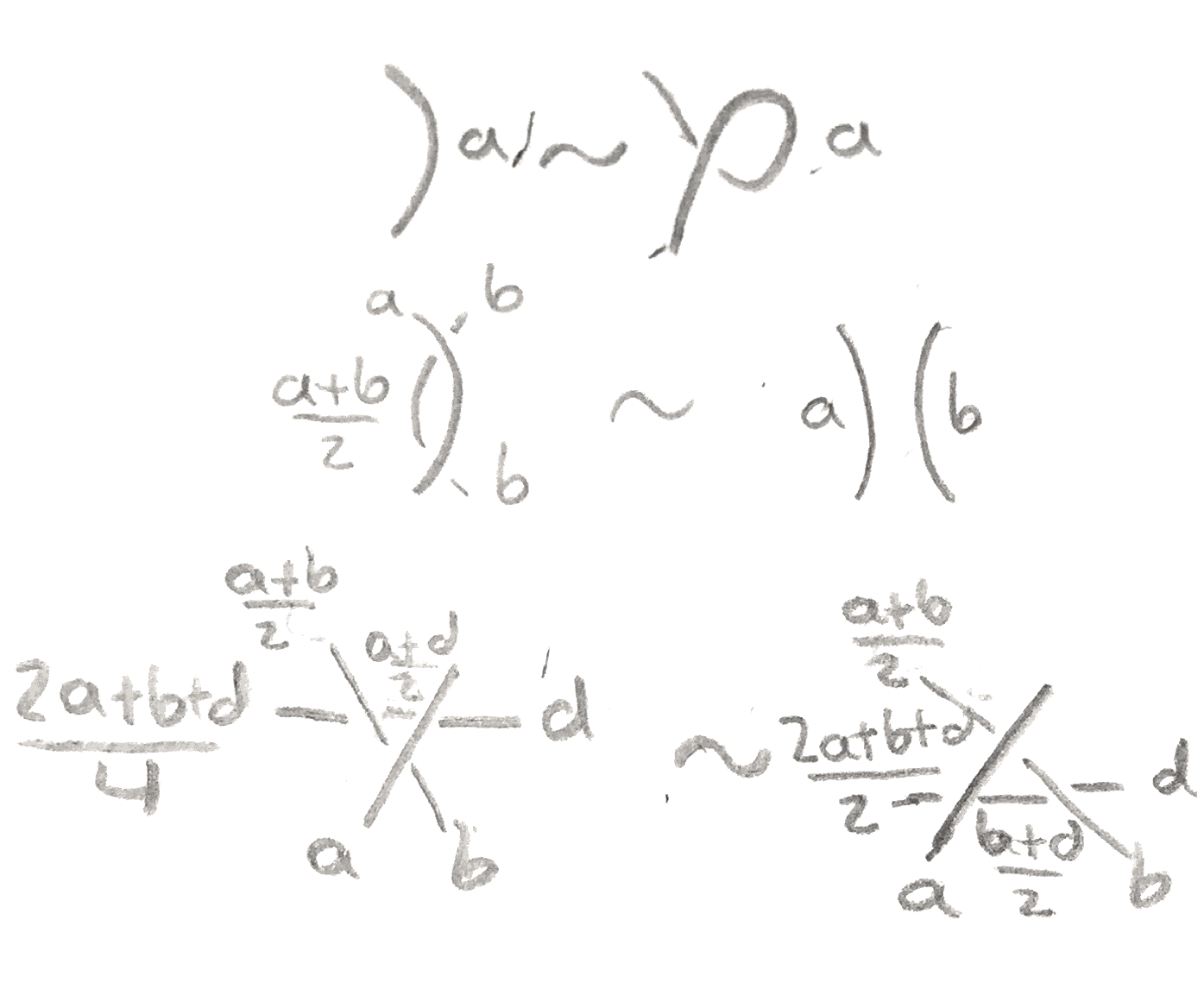
moves. Here is an example of one way to do that. We say that a link is \(3\)-colorable if we can give
each arc in the diagram one of three colors such that all colors are used, and such that at each
crossing the three different strands that meet either all have the same color, or all have different
colors. The pictures below show that our ability to \(3\)-color is invariant under the Reidmeister
moves:
Figure 3:A proof that \(3\)-colorability is an invariant of a link.
Moreover, the trefoil is \(3\)-colorable, and the unknot is not, so we have proved:
Theorem 1.1.The trefoil knot is not the same as the unknot.
Another link invariant the crossing number, or the smallest number of crossings that a knot
can possibly have. This, unlike \(3\)-colorability, is not as easy to compute, but has the property that
the only crossing number \(0\) knot is the unknot.
However, there is a special type of knot for which it is not as hard to compute, the alternatingknots. These are the knots that have a diagram such that if we move along a strand of the knot,
the strand will alternate at each crossing between being over or under the perpendicular strand.
For example, the trefoil and the figure \(8\) knot are alternating, and indeed many small knots are (for
example those with crossing number less than \(8\)), but as the knots get more complicated, fewer
knots become alternating.
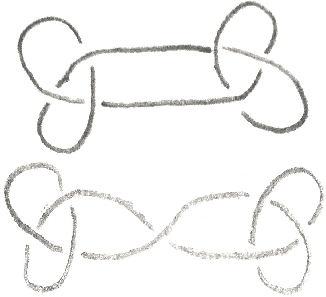
Namely, suppose we have a diagram for an alternating knot that is reduced, i.e. it has no
unnecessary crossings. An unnecessary crossing is one that separates the knot diagram
into two pieces. Here are some examples of alternating diagrams that are and aren’t
reduced:
Figure 4:The diagram on the top is reduced and alternating, and the diagram on the bottom
is alternating, but not reduced, as the crossing in the center separates the diagram into two
pieces. If we untwist that crossing, we get the diagram on the top.
Given an alternating diagram, we can make it become reduced by untwisting it at any crossing
that separates it into two pieces. It is easily seen that the resulting diagram is still alternating. It
was conjectured by Tait in the \(19^{th}\) century that a reduced alternating diagram of a knot has the
minimal number of crossings. The goal will be to prove this.
2. The Jones Polynomial
To prove this result, we will use a knot invariant called the Jones polynomial. It is a Laurent
polynomial in the variable \(t^{1/2}\), and for an alternating knot will be able to tell us the crossing number
of the knot.
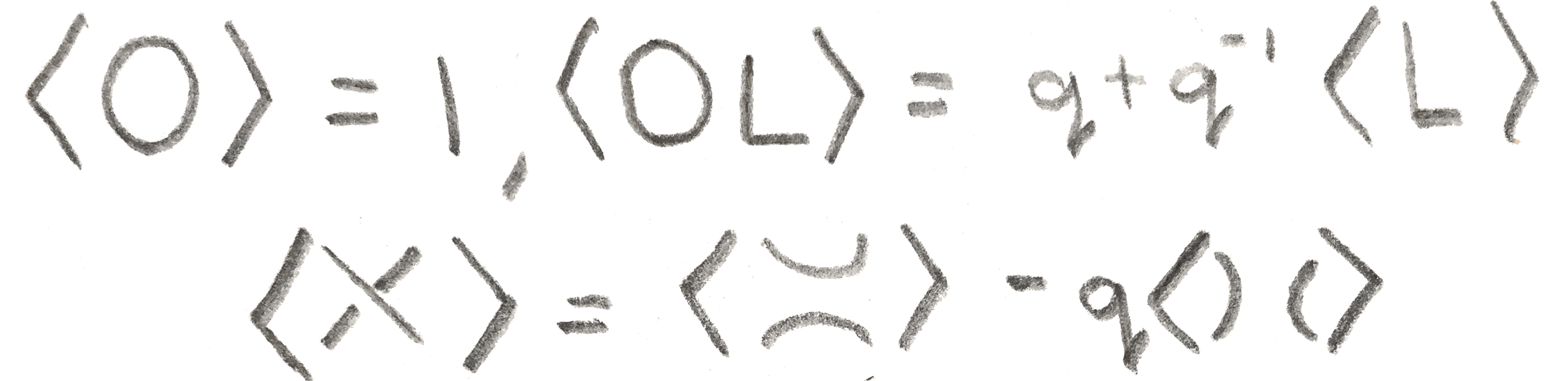
To construct the Jones polynomial, we will first construct the Kauffman bracket. This is only an
invariant of a diagram of the knot, not the knot itself. It is defined by the axioms shown
below:
Figure 5: The axioms defining the Kauffman bracket of a knot. In other words, the unknot
has bracket \(1\), adding a disjoint unknot multiplies the bracket by \(q+q^{-1}\), and “resolving” a crossing
of a link in two different ways gives a relation on the Kauffman bracket.
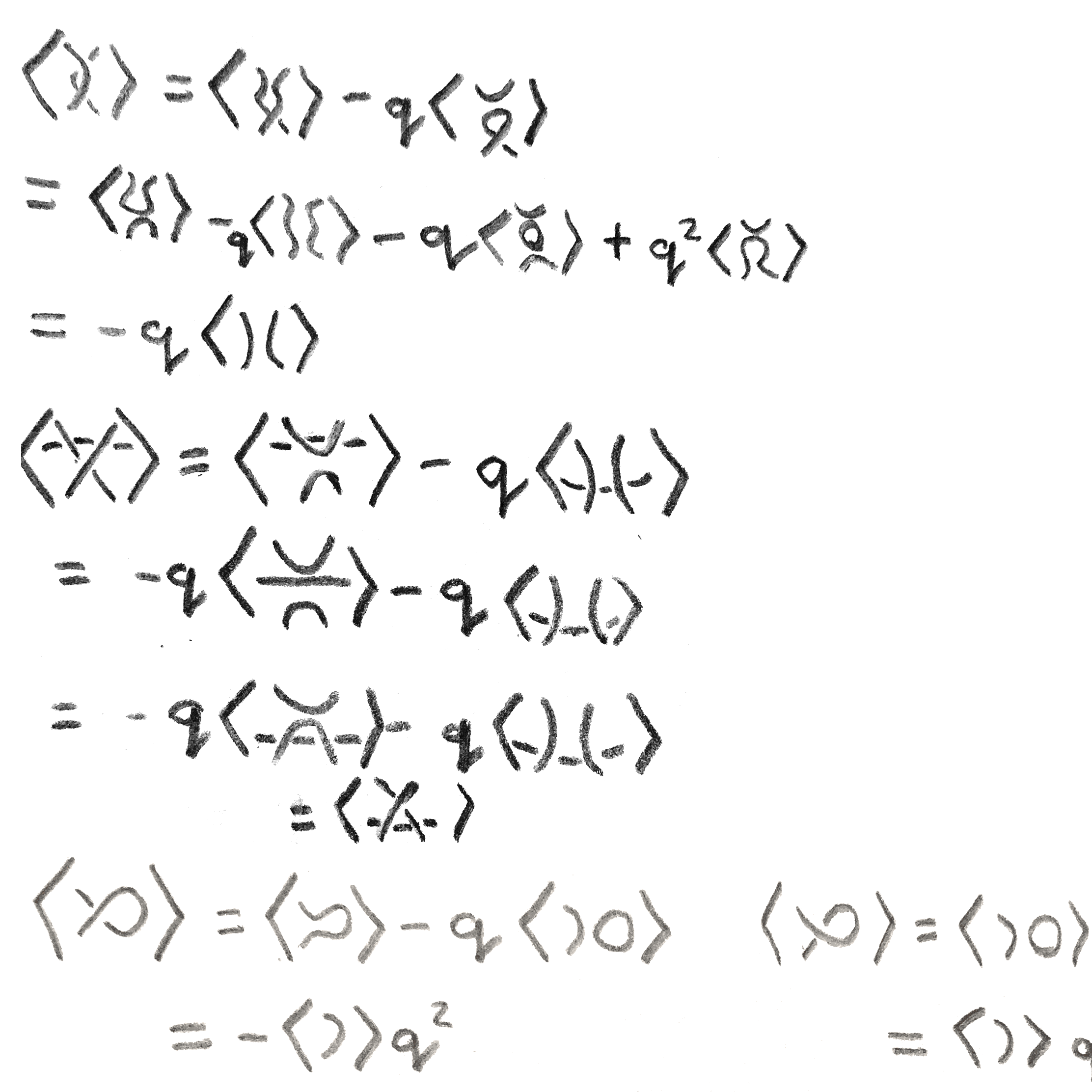
We can compute how it changes under the Reidmeister moves in Figure 6.
Figure 6: Shown above are computations to see how the Kauffman bracket changes with the
Reidmeister moves.
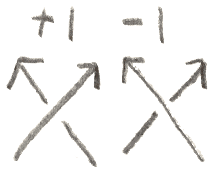
To get an actual knot invariant out of it, we must orient the knot \(K\), i.e. choose a direction to
move along the strand. Let \(n_+\) be the number of positive crossings, and \(n_-\) the number of negative
crossings. The convention to decide whether a crossing is positive or negative is shown in Figure
7.
Figure 7: Shown above is the convention for deciding whether a crossing of an oriented knot
is positive or negative.
Then by our computation of how the Kauffman bracket changes under the Reidmeister moves,
for an oriented knot \(K\) with diagram \(D_K\), the formula \(J(K)= (-1)^{n_-}q^{n_+-2n_-}\langle D_K\rangle \) gives a knot invariant of \(K\) called the Jonespolynomial of \(K\).
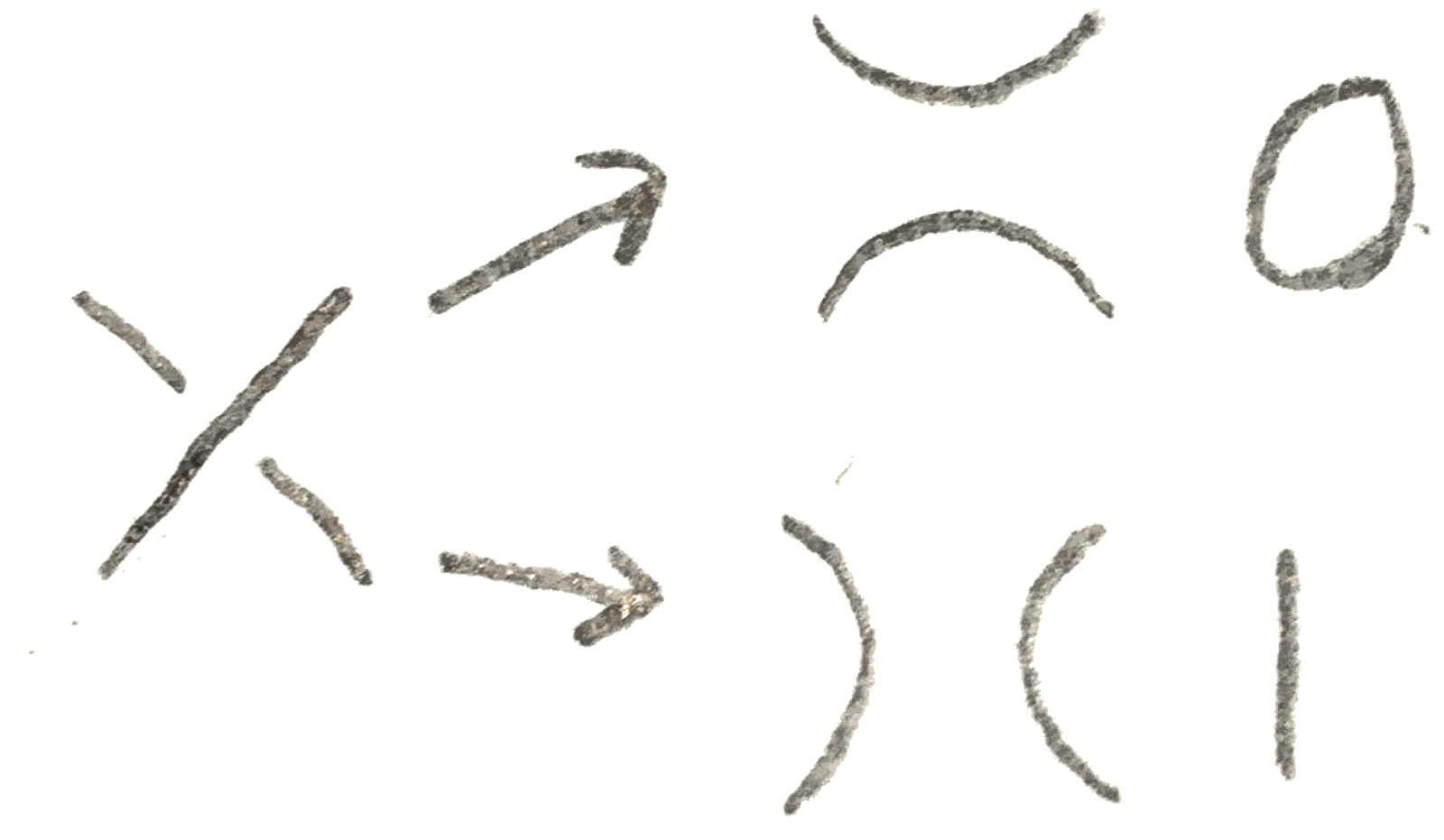
To compute the Jones polynomial, we consider all resolutions of the knot. Namely, crossing has
two resolutions, the \(0\) and \(1\)-resolutions, where we replace the crossing with one of the pictures shown
in Figure 8.
Figure 8: The two different types of resolutions.
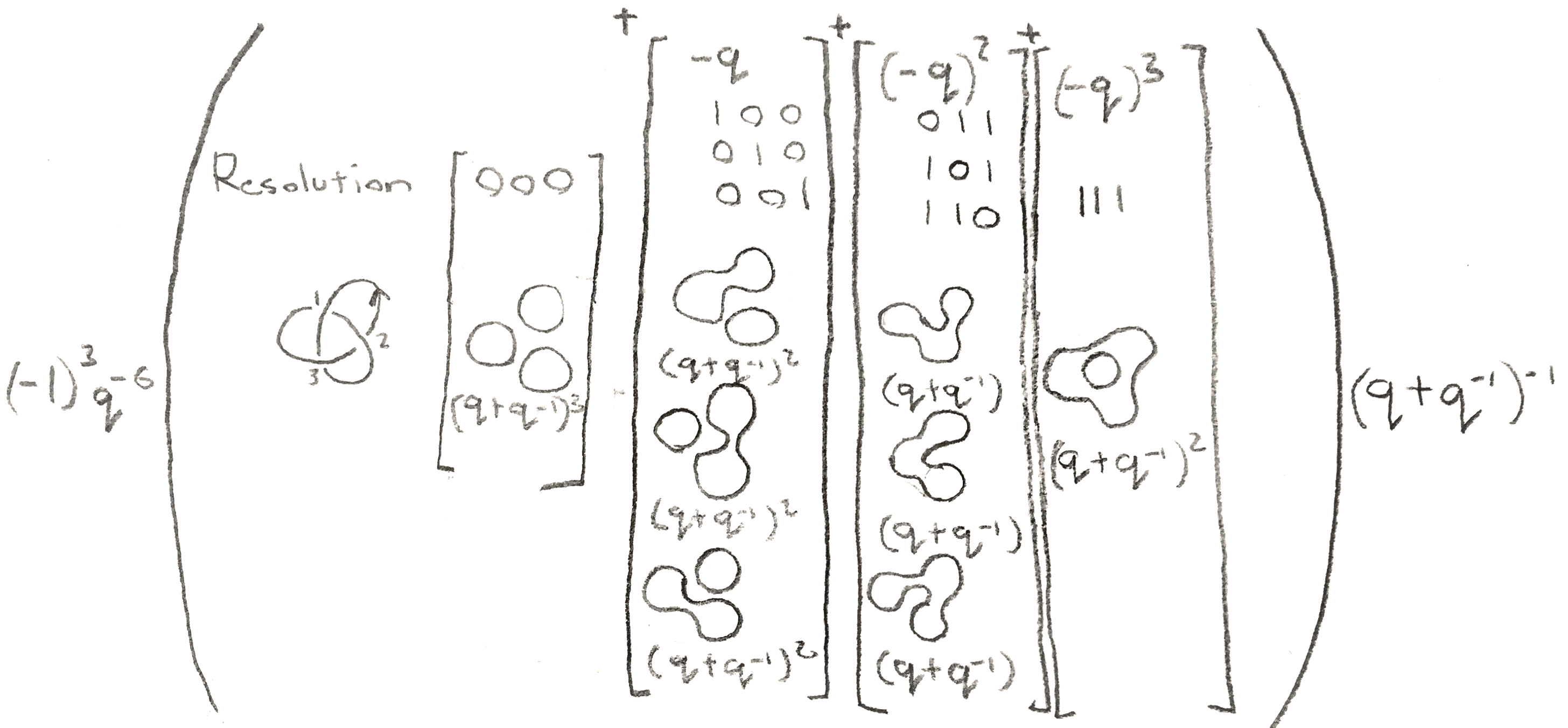
By looking at all possible resolutions and using the axioms, let’s compute the trefoil’s Jones
polynomial.
Figure 9: We compute the Jones polynomial of the left-handed trefoil from above as \(-q^{-6}((q+q^{-1})^2-3q(q+q^{-1})+3q^2-q^3(q+q^{-1})) = q^{-2}+q^{-6}-q^{-8}\).
The Jones polynomial tells us something about the crossing number of a link. Namely, let the
breadth of a Laurent polynomial \(p\) be the largest difference in exponent of nonzero terms in \(J(L)\), which
we will denote \(b(p)\). Note that if \(D_K\) is a knot diagram for \(K\), then \(b\langle D_K\rangle = b(J(K))\) is an invariant of the knot. We will soon
see that the breadth of the Jones polynomial generally gives a lower bound on crossing
number.
By looking at the Jones polynomial of the trefoil, we see that we must have \(c(3_1) = 3\), as \(6 = b(3_1) \leq 2c(K) \leq 6\).
This is a general phenomenon that holds for reduced alternating diagrams. The proof is to
examine carefully our computation for the trefoil, and see that the same kind of computation will
happen in any reduced alternating diagram. Namely, let us consider which terms can possibly
contribute the largest and smallest powers of \(q\) to the Jones polynomial. Certainly the
resolution consisting of only \(1\)s is always one of them. To see this, first note that as you
change the number of \(1\)s in the resolution, the number of unknotted components of the
resolution changes by exactly \(1\). Moreover, adding more \(0\)s will reduce the power of \(q\) that the
resolution contributes. Now two things very special happen for reduced alternating
diagrams.
Lemma 2.1.For a connected link diagram, the sum of the number of circles in theresolution with only \(1\)s and only \(0\)s is at most \(n+2\), with equality holding for an alternating diagram.In particular, \(b(J(K)) \leq 2c(K)\).
Proof.The second statement follows from the first, since if we resolve all the crossings, the
highest and lowest powers of \(q\) can come from the resolutions with only \(0\)s or only \(1\)s. Then there
are \(n+2\) circles in total for these two resolutions, and since there are \(n\) crossings, the difference in
\(q\) power that we get is \(n+2-1-1+n = 2n\), so \( 2c(K) \geq b(J(K))\).
For an alternating diagram, If suffices to prove that for each region that the knot diagram
divides the plane into, there is a unique circle in either the all \(1\)s or \(0\)s resolution that yields it.
If we consider the bounding circle on each region, since the knot is alternating, it coincides
with one of the resolutions of the knot. Moreover, since the boundary of each of the regions
touches each part of the knot twice, this gives a bijective correspondence.
More generally, for any connected diagram, we can prove this by induction on the number
of crossings. It is true for the standard unknot diagram, and if it is true for all connected
diagrams with \(< n\) crossings, and we have a diagram, with \(n\) crossings, we can choose any crossing,
and do its \(1\) and \(0\) resolution. Note first that by induction one of these yields a connected
diagram, say the \(0\)-resolution. Then let \(i_j\) denote the number of circles for the resolution where
on the first crossing we do the \(i^{th}\) resolution, and on the rest of the crossings we do the \(j^{th}\)
resolution. Then we have by induction that \(0_0+0_1 \leq n+1\) and \(|0_1-1_1|=1\) since they differ by one resolution. Then \(0_0+1_1 \leq n+2\).
□
Lemma 2.2.For a reduced alternating diagram, the resolution with all \(1\)s has morecomponents than the one with all but one \(1\)s, and similarly the resolution with all \(0\)s has morecomponents than all any with all but one \(0\).
Proof.The proof for the resolution with all \(0\)s is exactly the same, just use the knot where
all the crossings are switched. Now suppose that all the crossings are resolved with the \(1\)
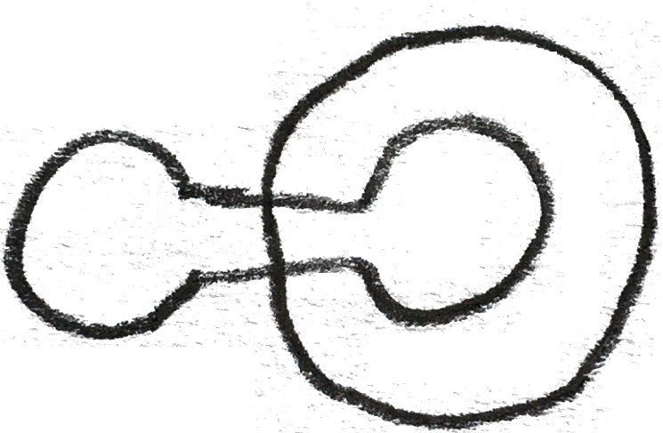
resolutions. Now suppose that there is a crossing that we can change that separates a region
into two regions. Then that circle looks like the circle below (we imagine it bounding the
region outside of it):
Figure 10: The circle at top (which we imagine as bounding the region of the knot outside
of it) splits into two when we change the resolution.
I claim that by doing the \(0\) resolution to this crossing, the knot becomes disconnected. This is
because since the two sides were originally in the same circle, and the interior of the circle is a
region not touching the knot, so there is a path not touching the knot going from one side of the
crossing to the other. Then by completing the path by making it intersect the crossing, we have
split our knot into two pieces, so it is not reduced.
Figure 11: In the situation above, we can draw a circle as shown here to split the knot into
two pieces, demonstrating that it isn’t reduced.□
Theorem 2.3.Let \(D_K\) be an alternating knot diagram for \(K\). Then \(D_K\) has the minimal number ofcrossings.
Proof.Because of Lemma 2.2, by looking at how each resolution contributes to the highest
and lowest terms of the Jones polynomial of \(K\), we see that there are no other terms that can
cancel them out. Then we see that the inequality in Lemma 2.1 is an equality. □
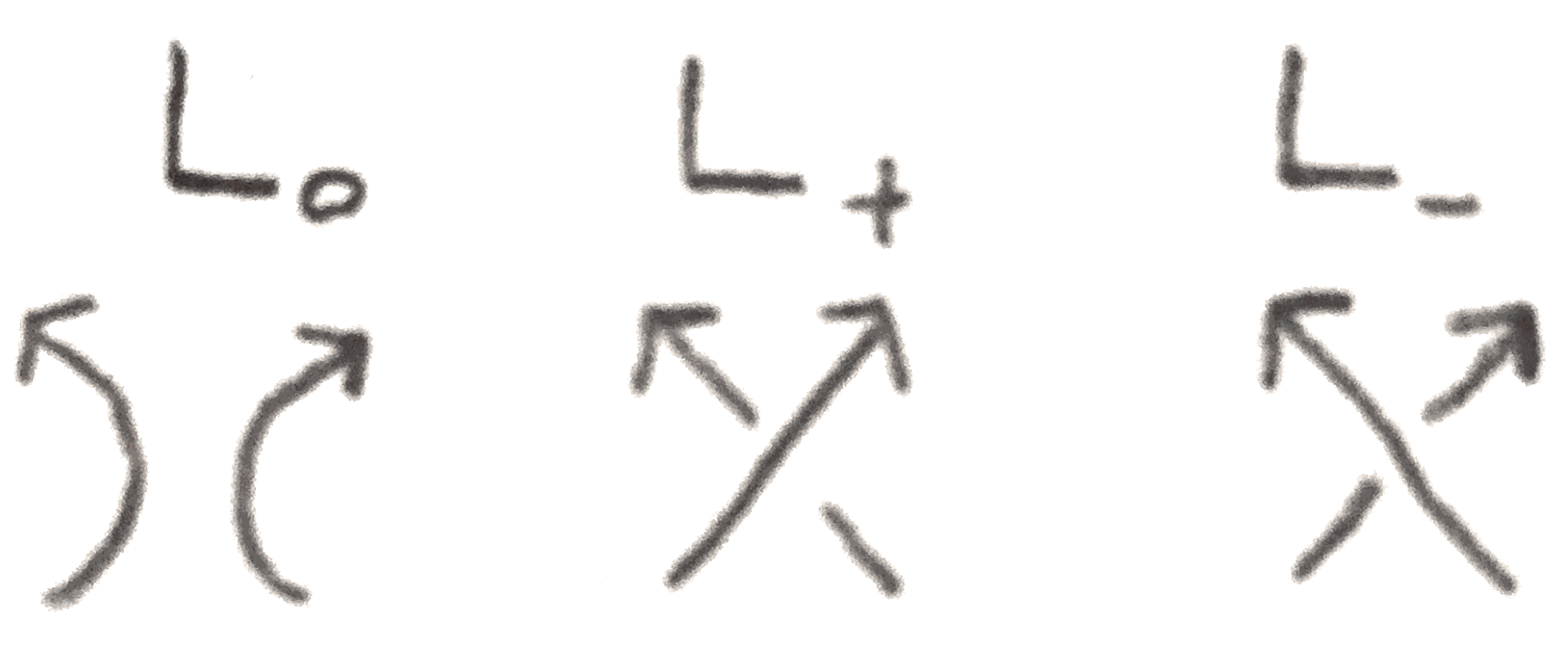
There is a faster way to compute the Jones polynomial. Namely, it satisfies the following relation
for \(3\) links \(L_0, L_+,L_-\) that look the same except near one crossing, they differ as shown in Figure
12:
Figure 12:
It follows from the axioms of the Jones polynomial that these satisfy the relation shown in
Figure 13:
Figure 13:
This can be used to compute \(J(8_{22})\) (with some orientation) more quickly, and the result is \(-q^2+2-q^{-2}+2q^{-4}-q^{-6}+q^{-8}-q^{-10}\). \(b(J(8_{22})) = 14 < 16 = 2c(8_{22})\), so it is
not an alternating knot.